Move from time to frequency
Use \(P(x,\omega)=\int p(x,t)e^{-i\omega t}\,dt\). A second time derivative becomes multiplication by \(-\omega^2\):
\[\mathcal F[p_{tt}]=-\omega^2P.\]So the wave equation becomes
\[-\Delta P-k^2P=S,\qquad k=\omega/c.\]COMPUTATIONAL ACOUSTICS · INDEPENDENT STUDY
An independent study following sound from an acoustic PDE to listening: finite elements, inverse problems, reduced models, interactive acoustics, modern music and historical recordings.
Recorded in wartime Vienna in December 1944, Furtwängler's Eroica later resurfaced as a controversial Urania LP, became the subject of a court case, and travelled through different tape, disc and digital-transfer lineages. The page follows that tangled history before asking how later editions changed what listeners actually heard.
1944 Vienna → Urania → Green Door / Tahra / Melodiya → listen to the three editions →


A large field guide to sound, perception, material, space and technology after 1911 — with composers, works, aesthetics, acoustic analysis and listening experiments.
NUMERICAL ROOM USED THROUGHOUT
Unless a section says otherwise, every result below uses this same 6 m × 4 m two-dimensional room.
This is intentionally a simple 2D model. It is useful for testing the numerical ideas below, but it is not a full model of a real concert hall or a vibrating structure.
WAVE EQUATION → HELMHOLTZ → FEM
We start with acoustic pressure in space and time. A Fourier transform lets us work one frequency at a time. Finite elements then replace the continuous pressure field by a finite list of nodal values.
The mesh has one unknown pressure value at each node. The matrix A(ω) tells us how those nodes are coupled at frequency ω; b is the source; solving the linear system gives the complex pressure field u.
The matrix used here is \(A(\omega)=K-k^2(1-i\eta)M\), with \(k=\omega/c\).
Use \(P(x,\omega)=\int p(x,t)e^{-i\omega t}\,dt\). A second time derivative becomes multiplication by \(-\omega^2\):
\[\mathcal F[p_{tt}]=-\omega^2P.\]So the wave equation becomes
\[-\Delta P-k^2P=S,\qquad k=\omega/c.\]Multiply by a test function \(\overline v\), integrate over the room, and integrate the Laplacian by parts:
\[\int_\Omega \nabla P\cdot\nabla\overline v-k^2(1-i\eta)\int_\Omega P\overline v=\int_\Omega S\overline v.\]Rigid walls mean \(\partial P/\partial n=0\), so the boundary term vanishes.
Write \(P_h=\sum_j u_j\phi_j\) and test with \(\phi_i\). This gives the stiffness matrix \(K\), mass matrix \(M\), and source vector \(b\):
\[[K-k^2(1-i\eta)M]u=b.\]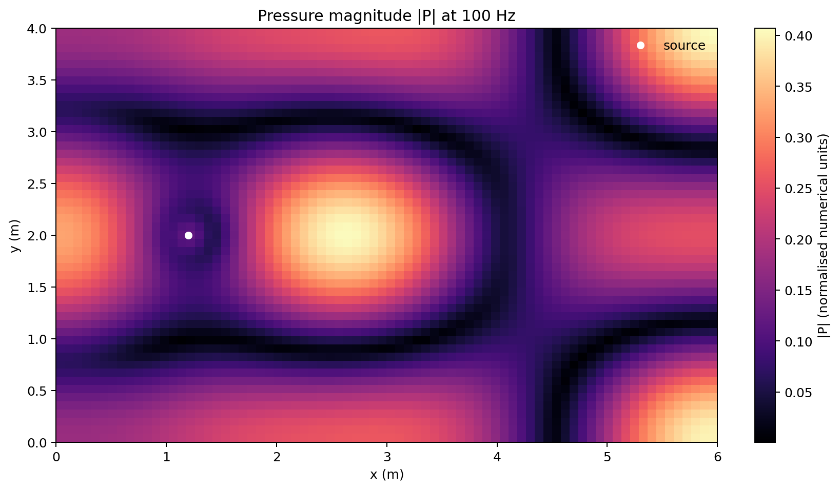
Before using the 2D room, the basic FEM assembly was tested on a 1D Helmholtz problem with a known solution. The error decreased approximately like \(h^2\) as the mesh was refined. This checks the implementation of the simple FEM machinery; it does not prove that the 2D room is a complete physical model.
At one frequency we need both amplitude and phase. A complex number stores both in one quantity. The physical time signal is real; the complex representation is a convenient frequency-domain description.
It gives a clean first model: no normal velocity through the boundary. Real concert-hall walls absorb and scatter sound in frequency-dependent ways, so this assumption is deliberately simplified.
A small phenomenological damping term. It keeps resonances finite. It is not a measured wall-loss model.
Because the goal is to make the numerical chain inspectable. A realistic hall would need 3D geometry, real boundary impedances and much more computation.
FIELD → LISTENING POSITION
For each frequency, we solve the pressure field in the whole room and then read the complex pressure at Seat A, Seat B and Seat C. Repeating this from 20 to 400 Hz gives one frequency-response curve for each seat.
Choose one frequency, for example 100 Hz.
Solve the whole room to get the pressure field at that frequency.
Read the pressure at A, B and C. Repeat for every frequency.
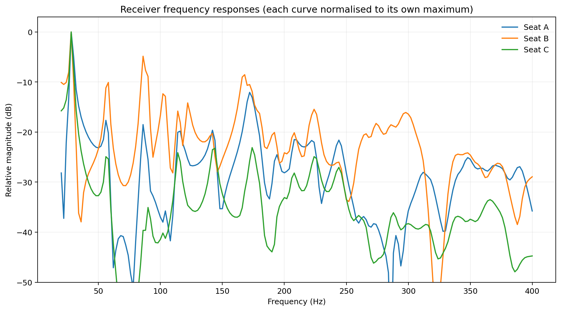
For one seat, \(H(f)\) is simply a frequency-by-frequency record of what the room does to the sound there: how much each frequency is changed in amplitude and phase.
For a linear time-invariant model, the output spectrum is the input spectrum multiplied by the room response:
\[Y(f)=H(f)X(f).\]The inverse Fourier transform of \(H\) is the impulse response:
\[h(t)=\mathcal F^{-1}[H(f)].\]The same operation in time is convolution: \(y=h*x\).
The computed response only covered 20–400 Hz. It was interpolated, tapered near the band edges and transformed back to time. Because the frequency spacing is 2 Hz, the corresponding periodic time window is \(1/\Delta f=0.5\) s.
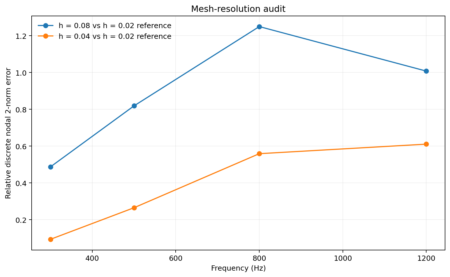
Higher frequencies have shorter wavelengths. If the mesh spacing stays fixed, fewer mesh points describe each wavelength, so the numerical solution becomes less reliable.
The note contains only its first three harmonics. This makes the change in harmonic balance easy to hear without presenting it as a full-band room simulation.
In this three-harmonic test, A has the weakest upper harmonics and sounds darkest; B has the strongest second harmonic and sounds brightest; C lies between them. Each seat is normalised to its own fundamental, so this compares colour rather than loudness.
REAL CONCERT HALLS
Yes. Our small 2D room cannot tell us where to buy a ticket, but the basic question is real: move the listener and the balance of direct sound and reflections changes. Real hall studies therefore measure many source and receiver positions rather than one single “room response”.
They are almost opposite answers to the same problem. Amsterdam's Concertgebouw is a late-19th-century shoebox: long, rectangular, stage at one end, and designed before modern room-acoustics science existed. Hamburg's Elbphilharmonie is a 2017 vineyard: the stage sits near the centre and the audience climbs around it in terraces. Both are famous, but they create and distribute reflections in very different ways.
Why it is unusual: its Main Hall became famous before acousticians had modern measurement tools or computer models. The Concertgebouw says the design borrowed from successful older halls, especially Leipzig's old Gewandhaus, and later renovations tried to preserve the original geometry and finishes.
What that means acoustically: the long parallel side walls of a shoebox send strong reflections back toward the audience. The Concertgebouw's own history describes a characteristically warm sound and an occupied reverberation time of about 2.2 s.
Seat position still matters: Bradley's 1991 measurements of the Concertgebouw, Vienna Musikverein and Boston Symphony Hall explicitly studied how acoustic quantities changed when the source or receiver moved.
Why it is unusual: the audience surrounds the stage and no seat is more than about 30 m from the conductor. Nagata Acoustics broke the audience into small terraces, designed reflecting surfaces around those terraces, and tested the hall with a 1:10 physical model. More than 10,000 individually milled “white skin” panels scatter and redirect sound.
Why people call it revealing: the hall's own acoustics guide describes the sound as very transparent and says that tiny details are easy to hear — including a fluffed note or audience noise. So the listener comment that the hall can feel “almost too revealing” has a real acoustic basis; the phrase “too good” is subjective, but the transparency is not invented.
Seat position is especially obvious: the official guide says seats beside or behind the stage can emphasise whichever instrument group is nearest, while higher seats tend to give a more balanced overall impression.
A classic hall whose successful acoustics were refined largely by experience and later measurement.
A modern hall whose geometry and surfaces were deliberately engineered to bring a large audience close to the stage.
There is no single universal “best seat”. A close seat may give more detail; another position may give a smoother blend or stronger sense of space. The best answer depends on the hall, the music and what the listener values.
No. A peak means that frequency is strongly amplified relative to the rest of that seat's response. A good seat is not defined by one large resonance.
To compare spectral shape. It deliberately removes absolute level differences, so the plot cannot tell us which seat is loudest.
At a given frequency, direct and reflected waves arrive with different phases. Changing position changes how they add or cancel, so peaks and dips move.
This was a small numerical demonstration. At higher frequencies the wavelength becomes shorter and the mesh would need to become much finer, which is exactly what the resolution audit shows.
MEASUREMENTS → UNKNOWN RESPONSE / FIELD
A forward problem starts with a model and predicts what microphones would measure. An inverse problem starts with measurements and tries to infer something we did not measure directly.
Known: room + source
Compute: microphone signal
Known: microphone signal
Infer: response or whole field
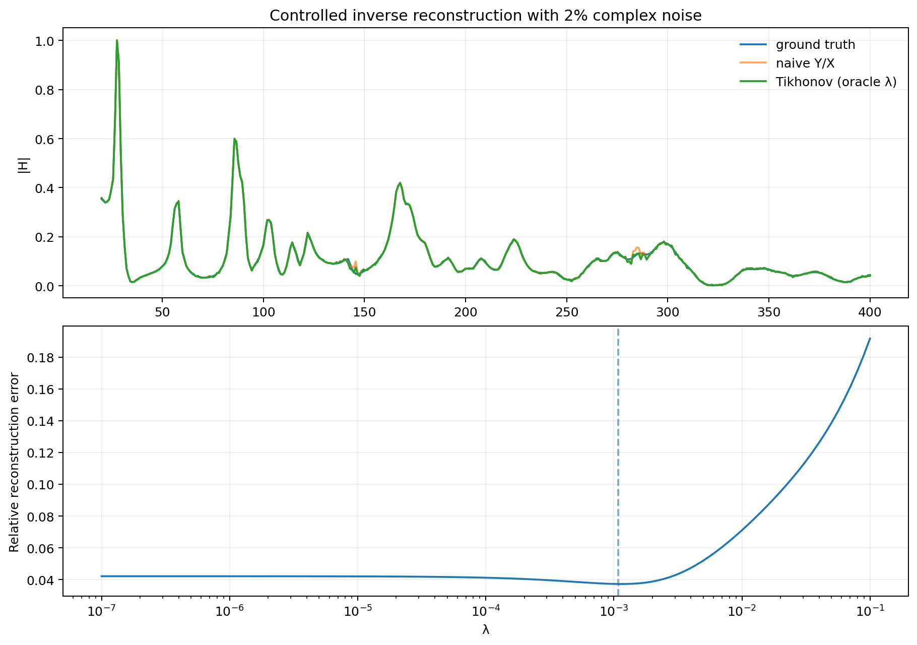
Suppose the input spectrum \(X\) is known and the measured output is \(Y=HX+\varepsilon\). The tempting estimate \(H=Y/X\) becomes unstable wherever \(|X|\) is very small, because the noise is divided by a tiny number.
Larger \(\lambda\) suppresses the instability more strongly, but also shrinks the estimate and introduces bias.
Suppose the FEM field has 15,251 nodes. Eight microphones give us only eight numbers at one frequency. We clearly cannot treat all 15,251 pressures as unrelated unknowns.
We have already solved this same room at many nearby frequencies. Those fields look different, but they are not random: the same kinds of spatial shapes keep reappearing. POD learns a small set of whole-room patterns that can be mixed together to describe those familiar fields.
40, 45, 50, …, 380 Hz. Each map contains 15,251 complex nodal values.
Think of them as spatial building blocks. Each block already covers the entire room.
In this project we keep 40 patterns. A familiar field is then described by 40 weights instead of 15,251 separate nodal values.
Plain English: the columns of \(V_r\) are the 40 whole-room patterns; the entries of \(a\) are the 40 mixing weights. Multiply each pattern by its weight and add them together to get an approximate field.
Write each full FEM field as one long column of 15,251 values. Put the 69 columns side by side. That table is the snapshot matrix \(U\).
We factor the snapshot matrix as \(U=V\Sigma W^*\). You do not need to think of this as a new physical model. It is a linear-algebra tool that finds directions that repeatedly appear in the snapshot data and orders them by how much of the snapshot variation they capture.
Each column \(v_i\) has one value at every FEM node, so each \(v_i\) is itself a complete spatial pattern over the room.
With \(r=40\), \(V_r=[v_1,\ldots,v_{40}]\). This collection of 40 columns is the POD basis used later in both sparse reconstruction and the reduced-order model.
The singular values in \(\Sigma\) tell us how much of the snapshot dataset is represented by the leading patterns. In this website that is a Euclidean coefficient-norm compression measure; it is not physical acoustic energy.
We want a simple repeatable layout, not a claim of “optimal microphone placement”. Start near the centre. Each time we add a microphone, put it at the candidate point that is currently farthest from all microphones already chosen. This avoids wasting many sensors in the same corner.
Pick a starting point.
Look for the place farthest from the microphones we already have.
Put the next microphone there.
Repeat, so the sensors gradually cover the room.
8 ⊂ 16 ⊂ 32 ⊂ 64
The formal name is farthest-point selection. The 8-, 16-, 32- and 64-microphone layouts are nested: the larger set keeps all microphones from the smaller set.
This is the important simplification. The microphones are not trying to guess every pressure value in the room directly. They only help us choose the 40 weights that best reproduce the measured microphone values.
What we actually know.
How much of each POD pattern?
Build an approximate whole-room field.
Nothing mysterious: \(C\) simply picks out the rows of a whole-room field that correspond to microphone positions. So \(CV_ra\) means “build the field from the POD patterns, then read that field only where the microphones are”.
We choose the weights \(a\) so that the predicted microphone values are close to the measured values \(y\), while a small regularisation term keeps the fit from becoming unstable in noise.
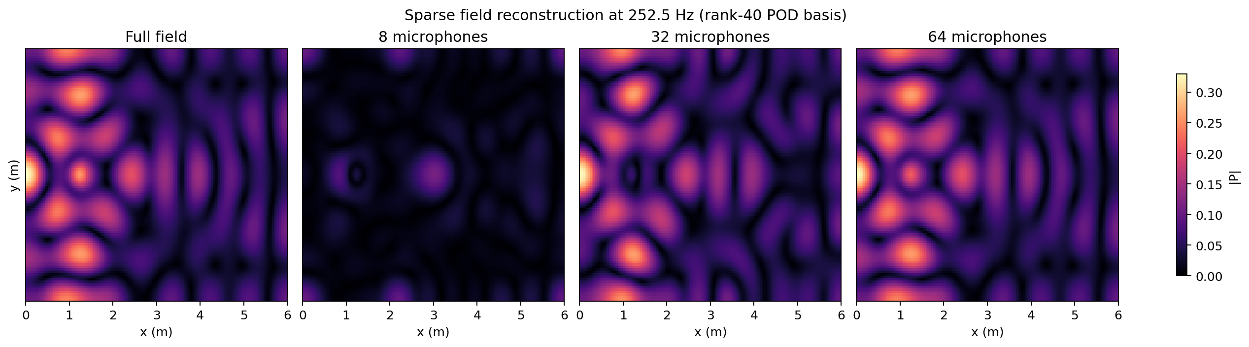
A reconstructed field can match the measured points very well and still be wrong in the spaces between them. We care about the whole field, so the final comparison must be made against the full FEM field, not only against the sensor readings.
Imagine 40 sliders but only 8 readouts. Many different slider settings can produce the same 8 numbers. In linear-algebra language, there is a nullspace.
Forty readings for forty weights leaves no spare information. If two POD patterns happen to look similar at those microphone positions, or if the measurements contain noise, a small error can cause a large change in the recovered weights. This is what “poor conditioning” means in practice.
Extra microphones give redundant information. Instead of forcing 40 equations to determine 40 weights exactly, we can find the set of weights that best fits many measurements at once, which is usually more robust to noise.
No. It works well in this one example with this basis, layout, frequency and noise level. A bad sensor layout can still miss important information, and optimal sensor placement is a separate research problem.
THE SAME POD PATTERNS, USED EARLIER
Section 03 used microphone data to choose the 40 POD weights. Here we ask a different question: can the Helmholtz equation itself choose those 40 weights, so we never have to solve for all 15,251 nodal pressures online?
The measurements choose the recipe.
The governing equation chooses the recipe.
The computer solves for every nodal value in \(u\).
The computer solves only for \(z_1,\ldots,z_{40}\), then rebuilds the field.
Plain English: we assume the new field can be made from the same 40 spatial building blocks learned from the snapshot fields. The only unknowns are how much of each block to use.
The full unknown vector \(u\) has 15,251 entries on this mesh.
Now the field is controlled by only 40 numbers in \(z\).
This is the Galerkin projection. A useful plain-language picture is: after choosing only 40 allowed building blocks, we make sure the remaining equation error has no component along those same 40 directions.
The online system is now 40 × 40 rather than 15,251 × 15,251.
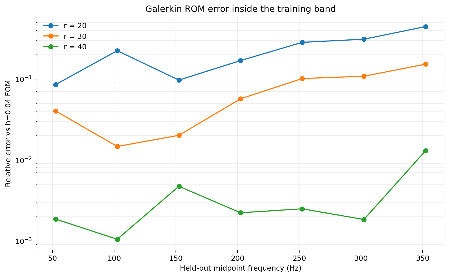
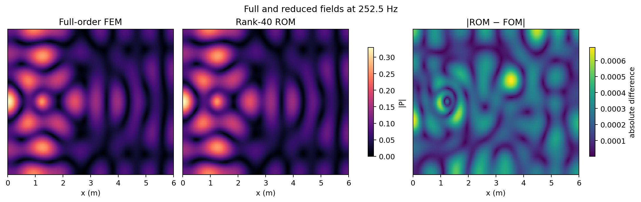
It saves online algebra: 40 unknown weights instead of 15,251 nodal pressures. It does not improve the mesh, change the PDE, or repair any error already present in the full FEM model.
POD gives us a reduced coordinate system: the 40 building blocks. In Section 03 we still used full solved fields to learn those blocks and then used microphone data to infer their weights. A Galerkin ROM goes one step further and uses the blocks inside the governing equations before the full solve.
They play the same kind of role — both are weights on the POD patterns — but they come from different information. \(a\) is fitted to microphone measurements; \(z\) is solved from the reduced Helmholtz equations.
Near a resonance, a small change in frequency can cause a large change in the field. A fixed set of 40 patterns may then need extra patterns or more careful stability treatment to follow that rapid change accurately.
No. It only proves that the ROM reproduces the chosen full FEM model well. If the full model has modelling or mesh error, the ROM can faithfully reproduce that error too.
This is a small 2-D numerical room. It is not a model of a measured space.
When meshes are compared, h = 0.02 is only the finest mesh used here. It is not an exact answer.
The microphone test uses synthetic data. The reduced model is checked against the full FEM solve, not against a real room.
Structural vibration and a full 3-D room model are outside this study.
SOUND LAB · LIVE
Eight interactive experiments now connect harmonic structure, beating, temporal fusion, spectral deformation, nonlinearity, sound masses and spatial hearing to concrete listening questions.
Open Sound Lab ↗Timbre · perception · modern music · space